L-systems

December 09, 2019

Biologist Aristid Lindenmayer created Lindenmayer systems, or L-systems, in 1968 as a way of formalizing patterns of bacteria growth. L-systems are a recursive, string-rewriting framework, commonly used today in computer graphics to visualize and simulate organic growth, with applications in plant development, procedural content generation, and fractal-like art.

Several L-systems rendered — A rendering of several L-systems.

The following describes L-system fundamentals, how they can be visually represented, and several classes of L-systems, like context-sensitive L-systems and stochastic L-systems. Much of the following has been derived from Przemyslaw Prusinkiewicz and Lindenmayer's seminal work, The Algorithmic Beauty of Plants.

String Rewriting

Fundamentally, an L-system is a set of rules that describe how to iteratively transform a string of symbols. A string, in this context, is a series of symbols, like " $a$ " or " $ababaabaaaa$ ", and can be thought of as a word comprised of characters. Each rule, known as a production, describes the transformation of one symbol to another symbol, series of symbols, or no symbol at all. On each iteration, the productions are applied to each character simultaneously, resulting in a new series of symbols.

Productions in this rewriting system can be described with "before" and "after" states, often described as the predecessor and successor; for example, the production $a \longrightarrow ab$ represents that the symbol $a$ transforms into the symbols $ab$ on every iteration. The length of derivation, or the number of iterations, is represented by $n$ . Given a word $a$ and productions $a \longrightarrow ab$ and $b \longrightarrow a$ , the following illustrates how the word transforms over several iterations, from $n=0$ to $n=4$ .

\begin{aligned} &a \\ &ab \\ &aba \\ &abaab \\ &abaababa \\ \end{aligned}

Figure 1 Word a transforming over 4 iterations of an L-system with the productions a → ab and b → a.

Formalizing L-systems

L-systems are formalized as a tuple with the following definition:

G = \langle V, w, P \rangle

Where the components are:

$V$ , the alphabet, or all potential symbols in the string.
$w$ , the starting word, also known as the axiom, comprised of symbols from $V$ .
$P$ , a series of productions describing the transformations or rules.

The L-system in Figure 1 can be formalized by defining its axiom ( $w$ ) and a series of productions ( $p_{1}, ..., p_{n}$ ) as:

\begin{aligned} w &: a \\ p_{1} &: b \longrightarrow a \\ p_{2} &: a \longrightarrow ab \\ \end{aligned}

The alphabet of all valid symbols can be inferred. It is implied that a symbol without a matching production has an identity production, e.g. $a \longrightarrow a$ .

D0L-systems

This fundamental form of an L-system is described as a deterministic, context-free L-system, or D0L-system (or sometimes DOL-system). 0L-systems are context-free, meaning that each predecessor is transformed regardless of its position in the string and its neighbors. Deterministic L-systems always produce the same result given the same configurations, as there is only one matching production for each predecessor.

Graphical Representation of L-systems

L-systems can be represented visually via turtle graphics, of Logo fame. While L-systems are string rewriting systems, these strings are comprised of symbols, each which can represent some command. A turtle in computer graphics is similar to a pen plotter drawing lines in a 2D space. Imagine giving instructions to a pen plotter to draw a square: "draw 1cm. turn right. draw 1cm. turn right. draw 1cm. turn right. draw 1cm". Though plotters don't really have an orientation, an L-system's turtle can be represented by Cartesian coordinates $x$ and $y$ , and an angle $\alpha$ that describes its forward direction. From there, symbols in a string can represent commands to change the state of the turtle.

To move a turtle around in 2D, symbols must be chosen to represent movement and rotation. The symbols $F$ , $+$ and $-$ will be used here, as they are commonly selected for these commands in L-system interpreters. After deriving the result of an L-system using its production rules, the string can then be parsed from left to right, with the following symbols modifying the turtle state:

$F$ move forward by $d$ units while drawing a line.
$+$ rotate left by angle $\delta$ .
$-$ rotate right by angle $\delta$ .

The variables $\delta$ and $d$ are global values indicating the magnitude of each symbol's rotation or movement. In non-parametric L-systems, each symbol's rotation and movement magnitude is a constant in the system.

A directed line traversing a Cartesian graph — **Figure 2** Visualizing the movement of a turtle and the line it creates from parsing the above string. From The Algorithmic Beauty of Plants *Figure 1.5b*.

Following the line in Figure 2 from the bottom left corner, the string can be read as "forward, forward, forward, right, forward, forward, right..." and so on.

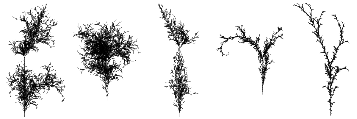
A tweet from @LSystemBot visualizing the L-System: {"start":"HHQ","rules":{"F":"[QN]F+F+","N":"[]++[HNQ]", "Q":"[F[]QFH++N]","H":"-FQNF[-]H"},"a":60,"iter":6} — An L-system generated by Twitter bot LSystemBot 2.0, tweeting an L-system and it's production rules every few hours.

A turtle may be decoupled from an L-system. The L-system has a starting string and a set of productions and outputs the resulting string. A turtle may take that final string as an input, and output some visual representation. For example, many of the illustrations shown here use the same L-system solvers, while using different turtles where appropriate, like one turtle built using CanvasRenderingContext2D and another using WebGL.

Space-Filling Curves

Space-filling curves can be formalized via L-systems, resulting in a recursive, fractal-like pattern. More specifically, FASS curves, defined as space-filling, self-avoiding, simple, and self-similar. That is, a single, non-overlapping, recursive, continuous curve.

\begin{aligned} \delta &: 90 \\ w &: X \\ p_{1} &: X \longrightarrow + Y F - X F X - F Y + \\ p_{2} &: Y \longrightarrow - X F + Y F Y + F X - \\ \end{aligned}

Figure 3 An L-system definition for a space-filling Hilbert Curve, animated over 7 iterations.

The Hilbert Curve (Figure 3) is an example of a FASS curve that can be represented as an L-system. Considered a Node-rewriting technique, this L-system's productions declare that on each iteration, $X$ and $Y$ symbols are replaced with more $F$ , $X$ and $Y$ symbols. With the angle $\delta$ defined as 90, this results in recursively generated square wave shape along a curve. While $F$ , $+$ and $-$ are interpreted by the turtle, other symbols can be used for productions. In this case, $X$ and $Y$ are ignored when rendering, and only relevant when rewriting the string and matching productions.

3D Interpretation

In addition to a turtle traversing on a 2D plane, symbols may be introduced that instruct the turtle to draw in 3D. The Algorithmic Beauty of Plants uses the following symbols to control rendering in three dimensions:

$+$ turn left by angle $\delta$ .
$-$ turn right by angle $\delta$ .
$\&$ pitch down by angle $\delta$ .
$\wedge$ pitch up by angle $\delta$ .
$\backslash$ roll left by angle $\delta$ .
$/$ roll right by angle $\delta$ .
$|$ turn around by 180°.

Like the 2D Hilbert Curve (Figure 3), a three-dimensional version can also be created (Figure 4) using these additional symbols, resulting in a 3D FASS curve.

\begin{aligned} \delta &: 90 \\ w &: X \\ p_{1} &: X \longrightarrow & \wedge \backslash X F \wedge \backslash X F \\ & & X - F \wedge / / X F \\ & & X \& F + / / X F \\ & & X - F / X - / \\ \end{aligned}

Figure 4 A space-filling Hilbert Curve from 1 to 4 iterations in 3D.

Bracketed L-Systems

The space-filling Hilbert curve can be represented as a single, continuous line. For organic, tree-like structures, branching is used to represent a diverging fork. Two new symbols, square brackets, are introduced to represent a tree in an L-system's string, with an opening bracket indicating the start of a new branch, with the remaining symbols between the brackets being members of that branch. Symbols after the end bracket indicate returning to the point of the branch's origin. A stack is used to implement branching, storing the state of the turtle on the stack.

$[$ push the current turtle state onto the stack.
$]$ pop the top state from the stack and this becomes the current turtle state.

Symbols in a branch are transformed and replaced just as they were outside of a branch. This allows recursive, fractal-like behavior, with each branch forking into more branches, and so on.

Figure 5 Animated branching L-systems, from 1 to 5 iterations. Definitions from The Algorithmic Beauty of Plants Figure 1.24.

Context-sensitive L-systems

Rather than productions evaluating symbols in isolation (context-free), rules may be defined that only matches a symbol when it proceeds or succeeds another specific symbol. Context-sensitive L-systems contain production rules that specify symbols that must come before or after the predecessor in order to match, as opposed to context-free systems that evaluate predecessors in isolation.

\begin{aligned} w &: baaaa \\ p_{1} &: b < a \longrightarrow b \\ p_{2} &: b \longrightarrow a \\ \end{aligned}

Figure 5 A context-sensitive L-system simulating signal propagation.

These context rules are defined using $<$ and $>$ in the production rule, adjacent to the predecessor. In Figure 5, the first production rule only matches when the $a$ symbol is immediately after $b$ , thus replacing the $a$ predecessor with its successor, $b$ . This results in the $b$ symbol moving towards the right:

\begin{aligned} &baaaa \\ &abaaa \\ &aabaa \\ &aaaba \\ &aaaab \\ \end{aligned}

A similar system could be defined that propagates $b$ from right to left, defined via production $a > b \longrightarrow b$ , replacing $a$ when there is a $b$ after it in the string.

Figure 6 Animated variants of context-sensitive L-systems, iterations 1 to 35. Definition from A model study on biomorphological description, illustrated in Figure 1.31 from The Algorithmic Beauty of Plants.

L-systems with these one-sided context productions may be considered 1L-systems. Productions may also have both a before-context and an after-context in systems considered 2L-systems. They can be represented as:

A < X > B \longrightarrow Y

This production rule indicates that the predecessor $X$ will be replaced by successor $Y$ when it is between an $A$ and a $B$ .

Stochastic L-systems

The previously described systems are all deterministic; the same system with the same input will always generate the same result. Stochastic L-systems are non-deterministic, defined by several productions that match the same predecessor, chosen randomly given their weight on each iteration. The following production rules define that on each iteration, $X$ has a 50% chance to be rewritten as $A$ , and a 50% chance to be rewritten as $B$ .

\begin{aligned} X & \xrightarrow{.5} A \\ X & \xrightarrow{.5} B \\ \end{aligned}

This non-determinism is useful for procedurally creating variety and the seemingly random results of nature.

\begin{aligned} w &: F \\ p_{1} &: F \xrightarrow{.33} F[+F]F[-F]F \\ p_{2} &: F \xrightarrow{.33} F[+F]F \\ p_{3} &: F \xrightarrow{.33} F[-F]F \\ \end{aligned}

Figure 7 A stochastic L-system animating over several variants. Definition from The Algorithmic Beauty of Plants Figure 1.27.